Ecological-Economic ContextThe QGIS plugin EcoValuator provides a simple means of estimating the dollar value of recreation, water supply, food, and other key ecosystem services for a given study area. Once installed, the tool combines satellite data on land cover with your own spatial data describing watersheds, conservation areas, townships, or other areas of interest.
The EcoValuator then does the work of estimating land area in each land cover type present in your region using the Benefits Transfer Method (BTM) to generate dollar-value estimates of the value of the ecosystem services supported by the land use/land cover present in your region*. *Not all combinations of land cover and ecosystem service are present in the literature, so EcoValuator will not provide estimates of the value of every service that could be flowing from every corner of your landscape. The absence of an estimate, therefore, should not be interpreted as an absence of value. We are grateful to the National Fish and Wildlife Foundation, whose generous support of Key-Log Economics’ research program “Ecosystem Services in the Roanoke River Basin” included creation of the EcoValuator. We also thank Philip Ribbens and Erich Purpur, who performed our original coding and updates to the plugin, respectively, and taught us all we know about creating and publishing QGIS plugins! Finally, we thank Maya Korb, who developed our User's Guide for Ecovaluator 3.0. |
Current coverage: North America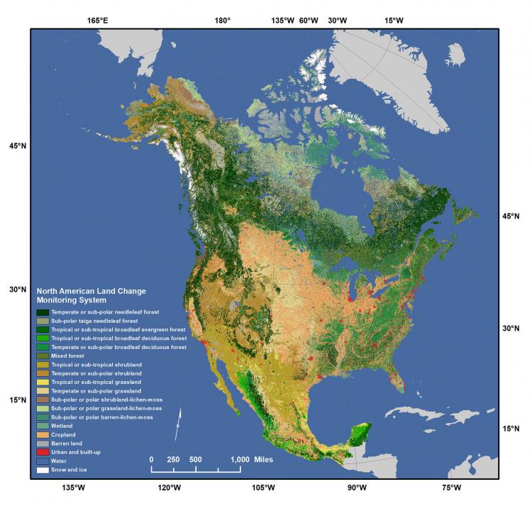
The EcoValuator currently supports land cover data from the National Land Cover Database (NLCD) and the North American Land Cover Monitoring System (NALCMS) (1,2). The NLCD classifies 16 land covers in the lower 48 states, while the NALCMS (pictured above) has 19 land cover classes spanning all of North America.
Resources
|
Ecosystem services are the effects on human well-being of the flow of benefits from an ecosystem endpoint to a human endpoint at a given extent of space and time (3).
This definition emphasizes that ecosystem services are not necessarily things–tangible bits of nature–but rather, they are the effects on people of those bits of nature. It also emphasizes that it is not just WHAT those effects are that matters: it is also WHEN and WHERE the effects occur. The “where” part, especially, is what drove us to create the EcoValuator as a tool for better understanding ecosystem service flows in one’s own region of interest.
Please see the tab at the far right for brief descriptions of ecosystem services we have included in the EcoValuator.
Benefit Transfer Method (BTM) provides an accessible way of estimating the value of ecosystem service flows in one setting (the policy area) based on the values estimated in another, similar, setting, called the “source” area. BTM is, in the words of the Organization for Economic Cooperation and Development, “the bedrock of practical policy analysis” when time and resource constraints preclude more involved methods (4).
In the EcoValuator, we employ a version of “unit value transfer” and apply estimates from a source study (or source studies) to the user-defined policy area based on matching land cover in both areas. Ecovaluator uses values from source studies compiled by the “TEEB” effort (for “The Economics of Ecosystems and Biodiversity” as well as those reviewed by Key-Log Economics in the course of our own ecosystem services assessments.
We began with an initial list of more than 1,200 specific estimates of the monetary value of specific ecosystem services arising from specific land cover types and then filtered out those for land covers not found in the conterminous United States, such as tropical rain forest, and polar and marine areas. We also excluded estimates from source areas where the nominal land cover might be similar, but where climate or other factors would make the estimates less applicable in the landscapes currently covered. Grasslands in Kenya, and wetlands in Vietnam are two examples. Finally, we excluded estimates from any source studies published before 1975.
We have classified each remaining source study estimate according to the ecosystem service (i.e., recreation, soil formation, water quality, etc.) and land cover type (open water, woody wetlands, etc.). We have also adjusted each value for inflation and for the relevant international currency exchange rates prevailing at the time of our latest update. That puts each value in units of 2018 dollars per hectare per year (2018$/ha/year).
Please see here for the final list of values and references to their associated primary studies.
Ecosystem Service |
Description |
Aesthetics |
Formation of landscapes that are attractive to people |
Air Quality |
Removal of contaminants from the air flowing through an ecosystem, including through filtration or decomposition |
Biodiversity |
The process of increasing genetic diversity across and within species |
Climate Regulation |
Modulation of regional/local climate |
Cultural, Other |
Non-material benefits people obtain from ecosystems through spiritual enrichment, cognitive development, reflection, and more, excluding recreation and aesthetics |
Erosion Control |
Control of the processes leading to erosion, for example, by controlling the effects of water flow, wind, or gravity. |
Food/Nutrition |
Ecosystems provide the conditions for growing food. Food comes principally from managed agro-ecosystems but marine and freshwater systems or forests also provide food for human consumption. |
Medicine |
Ecosystems and biodiversity provide many plants used as traditional medicines as well as providing the raw materials for the pharmaceutical industry. |
Pollination |
Contribution of insects, birds, bats, and other organisms to pollen transport resulting in the production of fruits and seeds. May also include seed and fruit dispersal. |
Protection from Extreme Events |
Extreme weather events or natural hazards include floods, storms, tsunamis, avalanches, and landslides. Ecosystems and living organisms create buffers against natural disasters, thereby preventing possible damage. |
Raw Materials |
Materials for construction and fuel including wood, biofuels, and plant oils that are directly derived from wild and cultivated plant species. |
Recreation |
Leisure and activity derived from ecosystems. |
Renewable Energy |
Resource utilization to produce renewable energy, specifically hydropower from open water. |
Soil Formation |
Process by which soil is created, including changes in soil depth, structure, and fertility. |
Waste Assimilation |
Removal of contaminants from the soil in an ecosystem, including through biological processes such as decomposition. |
Water Supply |
Filtering, retention, storage, and delivery of fresh water—both quality and quantity—for drinking, watering livestock, irrigation, industrial processes, hydroelectric generation, and other uses. |
How the ecovaluator works
The EcoValuator is really a pair of algorithms that the user runs sequentially. Users run the first step/algorithm ONCE for each region of interest, as defined by any polygon layer loaded into their QGIS project. The second step/algorithm can be then be run multiple times, with each run producing a new raster data set depicting the locations from a selected ecosystem service arises.
Step 1: Estimate ecosystem service values for study region
This algorithm does three things:
Once users have added the proper NLCD raster* and their study region polygon layer** to the QGIS project, they expand the “Key-Log Economics” and then the “EcoValuator” menu in the QGIS Processing toolbox and then click “Step 1: Estimate ecosystem service value for study region”. This algorithm has the following fields for the user to enter:
The input 2016 NLCD raster*: This is a copy of the National Land Cover Database (2016) depicting land cover in 16 types at the 30m resolution for the conterminous US. The NLCD raster that the user’s has added should appear in this drop-down.
Input mask layer (study region polygon layer)**: This vector data should describe the user's area of interest or study region. The algorithm clips the input NLCD data to this region.
Input table of ESV research data: This table of data comes pre-loaded with the plugin and provides the per-hectare-per-year minimum, average, and maximum dollar value estimates for each land cover type and ecosystem service. These figures are also adjusted for the exchange rate and inflation. These figures are derived from an extensive database (see Benefit Transfer Methods section).
Clipped raster layer: This output is the result of clipping process that is the first step of the algorithm.
Place to save intermediate file: If you'd like to save an html file with the number of pixels and total area (in m^2) for each different pixel value in the input raster [This is optional].
Output ESV table: This table contains NLCD land cover values and descriptions as rows, and associated ecosystem service values based on the minimum, mean, and maximum values per hectare from the ESV research data. Note that many NULL values will appear in the table due to a lack of existing research on certain ecosystem services in each land cover type, and NULL does not correspond to a dollar value of 0. It simply indicates a current lack of primary studies determine the dollar amount.
With the options chosen, the user clicks “Run in Background” to execute the process.
*Both the NLCD and input mask layer must be in CRS: ESPG: 102003 (https://espg.io/102003) (USA Contiguous Albers Equal Area Conic) in order to successfully execute the clip to the mask layer. Users can download a copy of the NLCD data in the proper CRS here.
- Clips the input land cover raster by the user-supplied Input mask layer for the region of Interest.
- Calculates how much area each type of land cover accounts for in the now-clipped land cover raster.
- Multiplies those areas by each of the associated per-hectare ecosystem service values (ESV) in the Input table of ESV research data.
Once users have added the proper NLCD raster* and their study region polygon layer** to the QGIS project, they expand the “Key-Log Economics” and then the “EcoValuator” menu in the QGIS Processing toolbox and then click “Step 1: Estimate ecosystem service value for study region”. This algorithm has the following fields for the user to enter:
The input 2016 NLCD raster*: This is a copy of the National Land Cover Database (2016) depicting land cover in 16 types at the 30m resolution for the conterminous US. The NLCD raster that the user’s has added should appear in this drop-down.
Input mask layer (study region polygon layer)**: This vector data should describe the user's area of interest or study region. The algorithm clips the input NLCD data to this region.
Input table of ESV research data: This table of data comes pre-loaded with the plugin and provides the per-hectare-per-year minimum, average, and maximum dollar value estimates for each land cover type and ecosystem service. These figures are also adjusted for the exchange rate and inflation. These figures are derived from an extensive database (see Benefit Transfer Methods section).
Clipped raster layer: This output is the result of clipping process that is the first step of the algorithm.
Place to save intermediate file: If you'd like to save an html file with the number of pixels and total area (in m^2) for each different pixel value in the input raster [This is optional].
Output ESV table: This table contains NLCD land cover values and descriptions as rows, and associated ecosystem service values based on the minimum, mean, and maximum values per hectare from the ESV research data. Note that many NULL values will appear in the table due to a lack of existing research on certain ecosystem services in each land cover type, and NULL does not correspond to a dollar value of 0. It simply indicates a current lack of primary studies determine the dollar amount.
With the options chosen, the user clicks “Run in Background” to execute the process.
*Both the NLCD and input mask layer must be in CRS: ESPG: 102003 (https://espg.io/102003) (USA Contiguous Albers Equal Area Conic) in order to successfully execute the clip to the mask layer. Users can download a copy of the NLCD data in the proper CRS here.
Step 2: Map the value of individual ecosystem services
This algorithm starts with the clipped NLCD raster and the ESV table generated in Step 1 and creates a new raster for which the value is the chosen per-pixel value (minimum, mean, or maximum) of the user-selected ecosystem service. The user can repeat this step for additional levels (min, mean, max) and/or additional ecosystem services.
To proceed, click “Step 2: Map the value of individual ecosystem services” in the QGIS Processing Toolbox. Users have the following options:
Input NLCD raster: This should be the output clipped raster from Step 1, an NLCD layer clipped by a region of interest.
Input ESV table: This should be the output ESV table from Step 1 and should not be altered.
The next two fields, “Ecosystem service of interest” and “ES value level”, specify the ecosystem service you want to map and whether you want to map minimum, average, or maximum values from the ESV table.
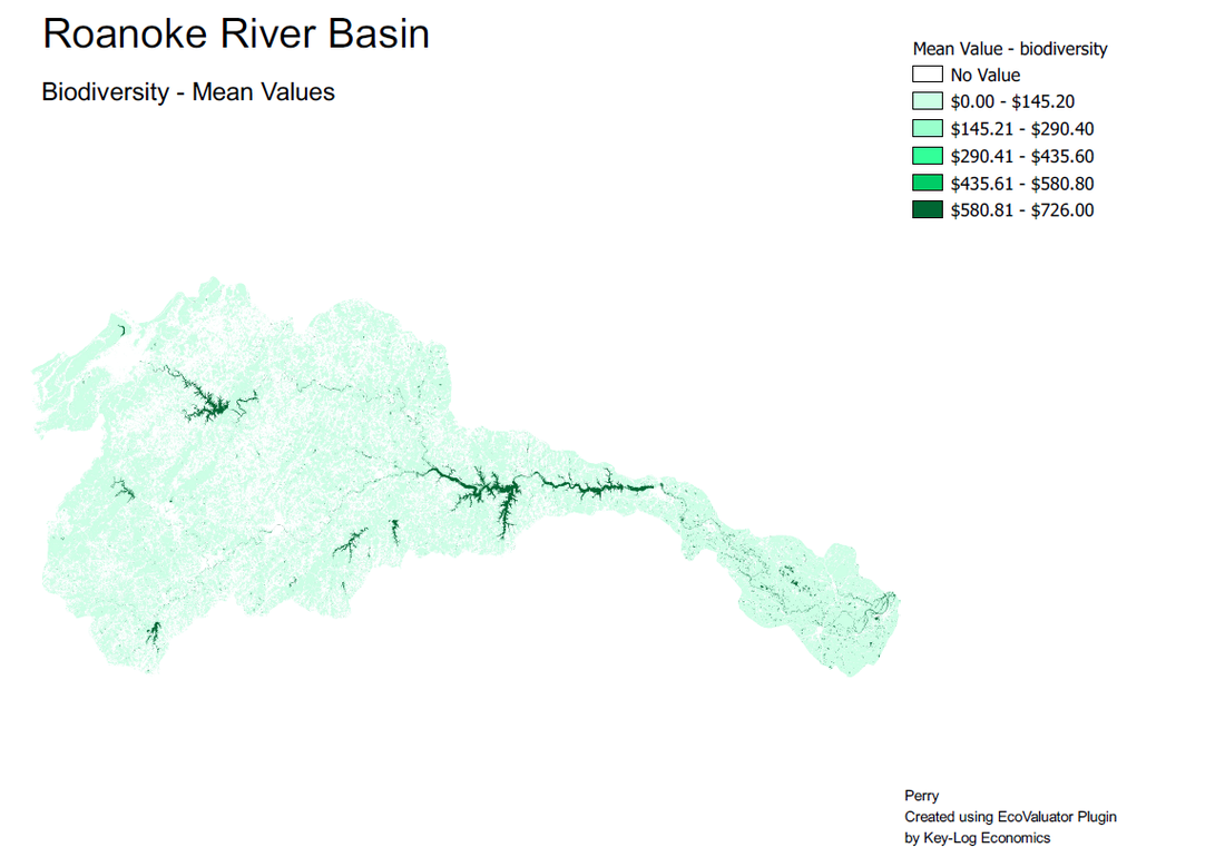
Step 3: Create print layout and export as .pdf
This step produces a finished map output as a .pdf. The output can contain the map, legend, title, subtitle, and credit text. Below is a sample output pdf for protection from extreme events (flood mitigation) in the Lower Roanoke River Basin.
Notes:
(1) Homer, C.G., Dewitz, J.A., Yang, L., Jin, S., Danielson, P., Xian, G., Coulston, J., Herold, N.D., Wickham, J.D., and Megown, K., 2015, Completion of the 2011 National Land Cover Database for the conterminous United States-Representing a decade of land cover change information. Photogrammetric Engineering and Remote Sensing, v. 81, no. 5, p. 345-354
(2) North American Land Change Monitoring System | Multi-Resolution Land Characteristics (MRLC) Consortium. (n.d.). Retrieved from https://www.mrlc.gov/data/north-american-land-change-monitoring-system
(3) Johnson, G. (2010, March). AIRES (Artificial Intelligence for Ecosystem Services) Workshop. Burlington, VT, USA: Gund Institute.
(4) Organization for Economic Cooperation and Development. (2006). Benefits Transfer. In Cost-Benefit Analysis and the Environment (pp. 253–267). OECD Publishing. Retrieved from http://www.oecd-ilibrary.org/environment/cost-benefit-analysis-and-the-environment/benefits-transfer_9789264010055-18-en